Supervised Clustering: How to Use SHAP Values for Better Cluster Analysis
Cluster analysis is a popular method for identifying subgroups within a population, but the results are often challenging to interpret and action. Supervised clustering leverages SHAP values to identify better-separated clusters using a more structured representation of the data. This article demonstrates the benefits of supervised clustering with an example based on simulated data. I provide a simple illustration of a methodology I applied to COVID-19 symptom clustering for a paper at the ECML PKDD 2021 conference.

The paper behind this article. Freely accessible here
This article assumes a basic understanding of SHAP, which is a technique for deconstructing a machine learning model's predictions into a sum of contributions from each of its input variables. If you'd like a general introduction to SHAP and how it can be used to understand the predictions of machine learning models, check out this guide.
Traditional Clustering Versus Supervised Clustering
Traditional approaches to clustering are quite simple, and are typically implemented as follows:
- Pre-processing is conducted to tidy and rescale the data
- Optionally, the data may undergo dimensionality reduction - typically to two dimensions, for visualisation purposes
- Clustering algorithms are applied, and various metrics are used to assess the quality of clusters that are identified
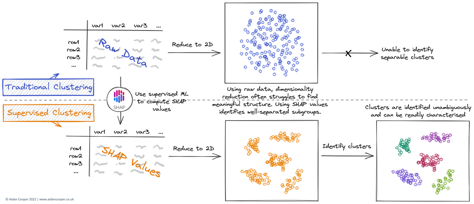
This often produces disappointing results, with poorly defined, strongly overlapping clusters that cannot be differentiated convincingly. Supervised clustering adopts a similar workflow, but with an additional step, as illustrated in Figure 1.
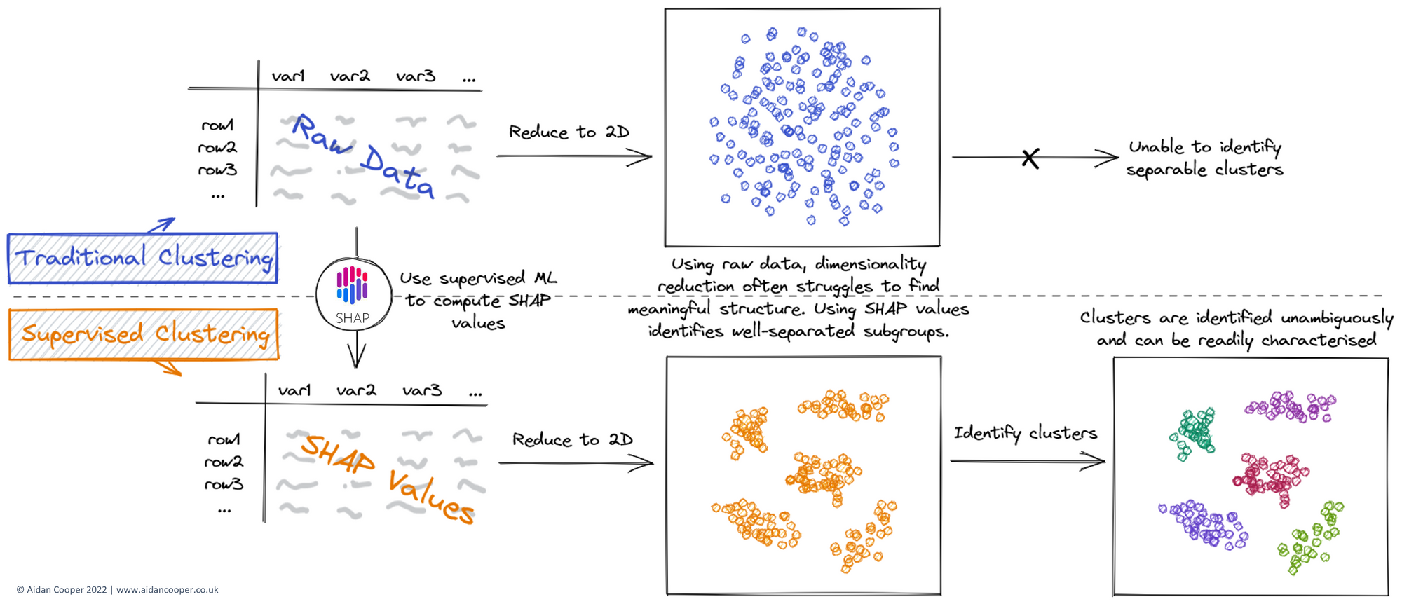
Rather than cluster on the raw data directly (or an embedding thereof), supervised clustering first converts the raw data into SHAP values. This involves using the raw data to train a supervised machine learning model, and then computing SHAP values with this trained model. The result is an array of equal dimensions to that of the raw data, but with values that are determined by how informative the data is in relation to the target variable.
For this to be possible, an essential prerequisite for supervised clustering is the presence of an appropriate target variable to use for training the prediction model. This is a strong departure from traditional cluster analysis, which is conventionally regarded as a fully unsupervised technique. Fortunately, many clustering applications naturally lend themselves to this process. For example, in our COVID-19 symptom clustering paper, we had patient symptom data (i.e. model inputs) which could be used to predict COVID-19 infection status (i.e. binary target variable), to allow us to identify subgroups of COVID-19 symptomatology (i.e. the clustering task).
The Advantages of Supervised Clustering
There are two interrelated benefits to using SHAP values for cluster analysis:
- Computing SHAP values serves as a pre-processing step that rescales raw data into common units (the output of the supervised prediction model). This elegantly handles the common challenge where we want to cluster data containing features with very different units and scales (e.g. dollars, metres, colour etc.)
- SHAP values weight the data by a measure of importance that emphasises the most informative features whilst minimising the influence of irrelevant features. Traditional clustering biases features based on the magnitude of their distributions, regardless of their actual information content. Using SHAP values de-noises the data of irrelevant information and amplifies features proportional to the signal that they generate.
These properties lead to supervised clustering producing highly-differentiated, characterisable clusters that are easy to discern and interpret.
Supervised Clustering: A Worked Example
A Simulated Dataset Containing Subgroups
To demonstrate the benefits of supervised clustering, we simulate a dataset of 1,000 instances and 50 features, and a binary target variable, y. Only the first 5 features are actually informative, with the remaining 45 being statistical noise. Using scikit-learn's make_classification function, we can also specify that the data has three clusters for each of y's binary values. These clusters are what we will aim to recover through our analysis.
For the supervised machine learning model, we train a gradient boosted tree with lightgbm that predicts y using the 50 features as inputs. This trained model is then used to compute SHAP values using the shap package.
import lightgbm as lgb
import shap
from sklearn.datasets import make_classification

# simulate raw data
X, y = make_classification(
    n_samples=1000,
    n_features=50,
    n_informative=5,
    n_classes=2,
    n_clusters_per_class=3,
    shuffle=False
)

# fit a GBT model to the data
m = lgb.LGBMClassifier()
m.fit(X, y)

# compute SHAP values
explainer = shap.Explainer(m)
shap_values = explainer(X)
Unlike in typical machine learning prediction workflows, we don't need to split the data, as our objective is merely to transform the 1,000x50 array of raw data into a new representation: a 1,000x50 array of SHAP values. This means we can simply fit the model directly to all the available data and ignore the possibility of overfitting.
Figure 2 visualises this data in both its raw and SHAP representations, constructed as violin plots for each feature. The left-hand, blue halves show the distributions of raw values, and the right-hand, pink halves show their corresponding distributions of SHAP values.
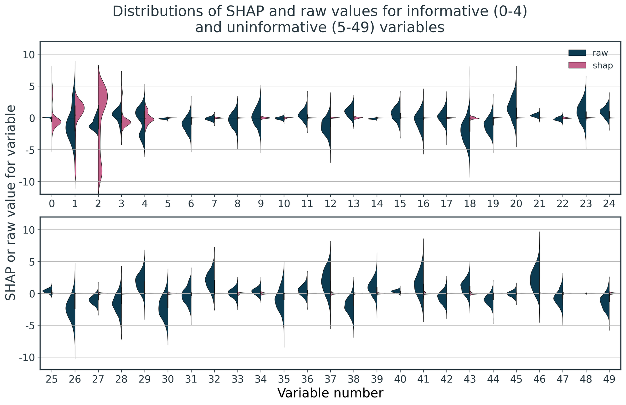
For the raw data, we see the features have distributions of values that vary in magnitude, but this is random and irrespective of their informativeness. By contrast, for the SHAP values, only the informative features, 0-4, have non-zero distributions. The SHAP values for the uninformative values have effectively shrunk to zero.
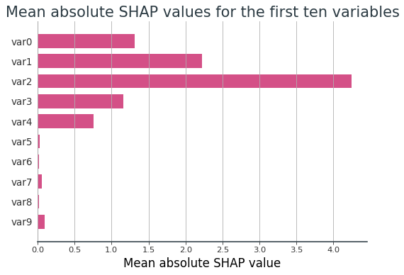
This can be confirmed by examining the mean absolute SHAP value of each feature, as presented in Figure 3. Using SHAP values, the informative features become scaled dependent on how influential they are on the supervised ML model's predictions, whereas all the uninformative features are disregarded. This effectively eliminates the influence of the uninformative features on the subsequent clustering.
Visualising the Raw Data and SHAP Values in Two Dimensions
Dimensionality reduction is a common but non-essential stage in many clustering workflows. It's popular for visualising clusters in two dimensions so that they can be assessed by eye, and we employ UMAP for this purpose in this example.
from umap import UMAP

# compute 2D embedding of raw variable values
X_2d = UMAP(
  n_components=2, n_neighbors=200, min_dist=0
).fit_transform(X)

# compute 2D embedding of SHAP values
s_2d = UMAP(
  n_components=2, n_neighbors=200, min_dist=0
).fit_transform(shap_values.values[:, :, 1])
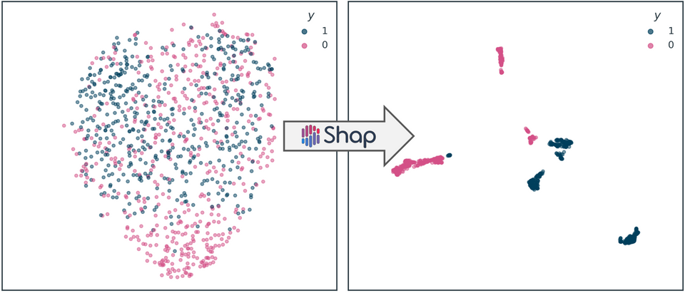
Figure 4 shows the 2D embeddings produced by UMAP when applied to the raw data and SHAP values. The raw data embedding contains little structure, with almost complete overlap between the two classes of the target variable, y. However, the SHAP values embedding clearly recovers each class' three underlying clusters (with minor inaccuracies in the case of one of the clusters).
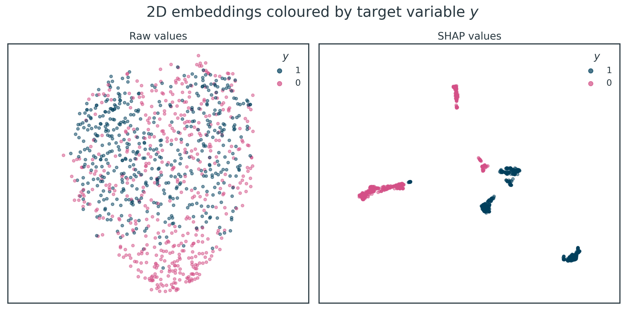
Depending on your use case for supervised clustering, you may want to apply dimensionality reduction to only one of the target variable's classes. For example, in our COVID-19 symptom clustering work, we were only interested in subgroups of COVID-19 symptomatology so we only clustered the patients with the positive COVID-19 infection status label. This may also be necessary if the underlying supervised machine learning model has poor predictive performance. In this toy example, the predictive model has high predictive power, and the corresponding SHAP values allow us to distinguish all six clusters across the two classes of y unambiguously.
Clustering the 2D Embedding of SHAP Values
The clusters are well separated for the 2D SHAP value embedding and could be readily identified by any number of clustering algorithms. In this example, we elect to use DBSCAN.
from sklearn.cluster import DBSCAN

# Identify clusters using DBSCAN
s_labels = DBSCAN(eps=1.5, min_samples=20).fit(s_2d).labels_
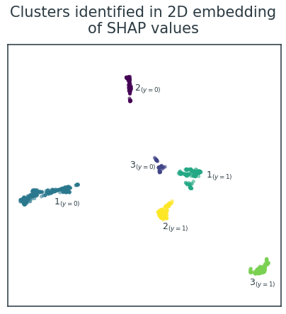
As expected, this identifies the same six clusters that can be discerned visually (Figure 5). I've manually labelled the three clusters associated with each binary class as \( N_{(y=m)} \) through comparison with Figure 4.
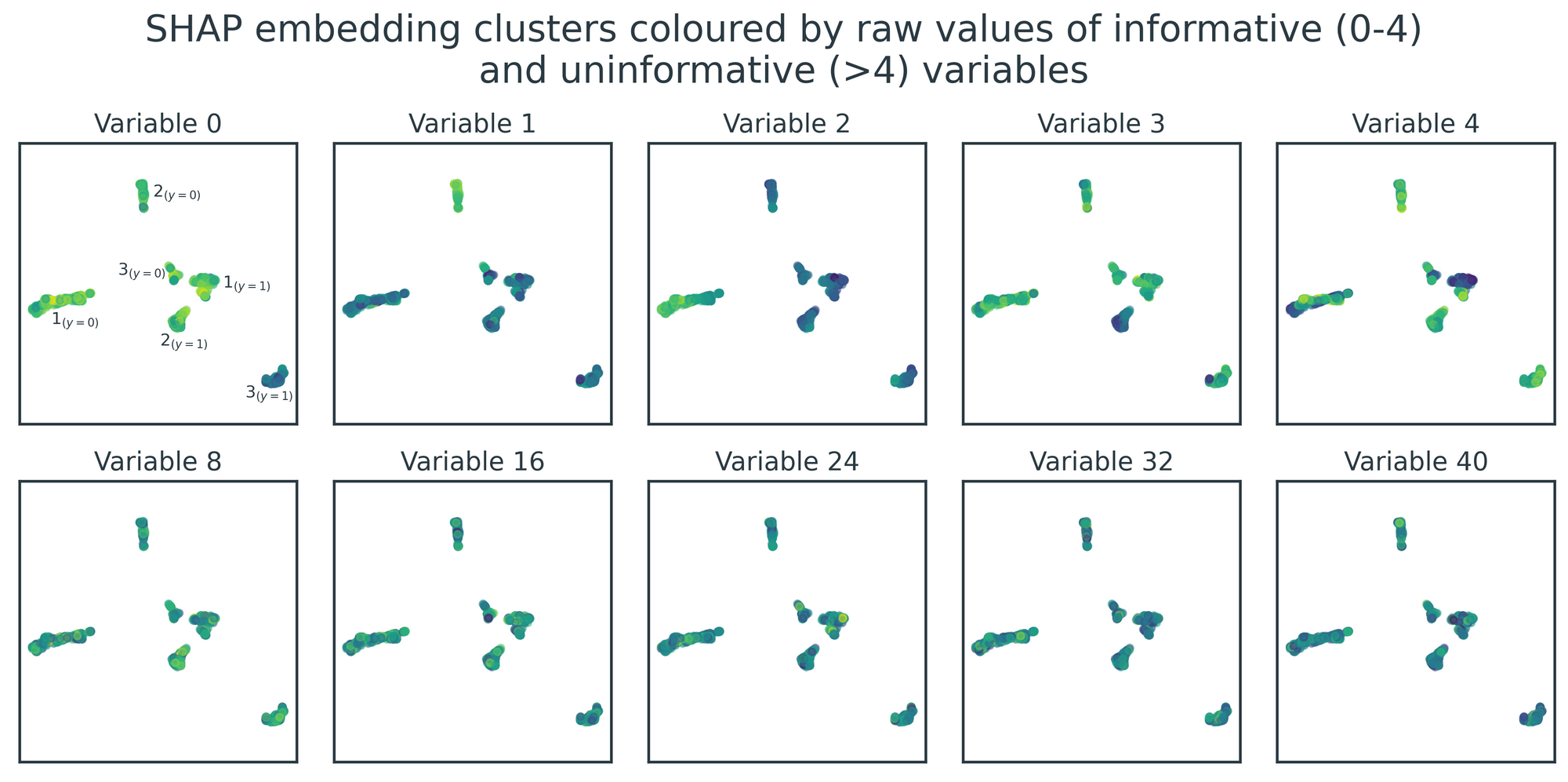
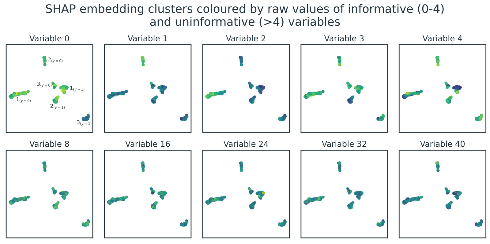
Crucially, even though these clusters are derived from SHAP values, they still hold meaningful relationships with the original raw data. Figure 6 visualises the relationship between the six clusters and the raw values of the five informative variables and five example uninformative variables. There are clear patterns for the informative variables, with individual clusters exhibiting homogeneity and some clusters possessing higher/lower variable values than others. Conversely, the clusters show no structure in relation to the underlying values of the uninformative variables.
Characterising the Clustered SHAP Values
We can take this a step further by succinctly characterising each cluster with decision rules using the SkopeRules package. We do this using a one-vs-all methodology, in which decision rules are learnt for each cluster in turn, that differentiates it from all the other clusters, using the original raw data as inputs. In doing so, we identify decision rules and characterise the clusters completely independently of the SHAP values that supported their derivation.
In this example, we ensure that the identified rules are very simple by enforcing that they can only be comprised of two comparison terms.
import numpy as np
from skrules import SkopeRules

for cluster in np.unique(s_labels):
    # create target variable for individual cluster
    yc = (s_labels == cluster) * 1
    # use SkopeRules to identify rules with a maximum of two comparison terms
    sr = SkopeRules(max_depth=2).fit(X, yc)
    # print best decision rule
    print(cluster, sr.rules_[0][0])
    # print precision and recall of best decision rule
    print(f"Precision: {sr.rules_[0][1][0]:.2f}",
          f"Recall   : {sr.rules_[0][1][1]:.2f}\n")
Table 1 reports the identified rules, and their corresponding precision and recall scores for differentiating each cluster from its five counterparts. Unsurprisingly, we can see that the identified rules only make use of the informative variables, 0-4. With the exception of \(3_{(y=0)}\), all the rules are effective at identifying instances that belong to their cluster. We could likely achieve higher performance across the board by allowing SkopeRules to generate more complex rules by increasing the max_depth parameter, or by using an ensemble of decision rules for each cluster.
| Cluster | Decision Rule | Precision | Recall |
|---|---|---|---|
| 1(y=0) | var0 > -0.05 and var2 > -0.71 |
93% | 99% |
| 2(y=0) | var1 > 2.34 and var4 > -1.42 |
98% | 97% |
| 3(y=0) | var0 > 0.12 and var2 < -0.78 |
54% | 36% |
| 1(y=1) | var2 > -0.76 and var4 < -1.62 |
93% | 79% |
| 2(y=1) | var3 < -0.89 and var4 > -1.51 |
92% | 88% |
| 3(y=1) | var0 < -0.04 and var3 > -2.10 |
96% | 91% |
Table 1. Cluster decision rules, based on raw variable values, and their associated precision and recall scores
We've achieved our goal of recovering the six ground-truth clusters in the simulated dataset and succinctly described them using decision rules. These rules can be confirmed visually by examining Figure 6 - for example, \(2_{(y=0)}\) is the only cluster that is bright in colour (i.e. high raw values) for both variables 1 and 4, consistent with its decision rule, var1 > 2.34 and var4 > -1.42.
Conclusion
In this article, I've demonstrated the benefits of supervised clustering by successfully identifying clusters for an example dataset where traditional clustering fails. These clusters were highly separated and characterised by interpretable decision rules, illustrating the practical utility of this approach.
Supervised clustering is a nascent technique, and there are subtleties involved in training the machine learning model and selecting hyperparameters for the algorithms used at each stage. Requiring a suitable target variable for model training is the main limitation of supervised clustering, although many use cases are a natural fit for this methodology.
The workflow outlined in this post is powerful and flexible, and I encourage the reader to experiment with it for their clustering tasks!
 AidanCooper
Code for this analysis can be found on GitHub


Member discussion