Approximating Shapley Values for Machine Learning

In a previous post, I explained the theory behind Shapley values. I also explained that calculating Shapley values for real world machine learning use cases is typically computationally infeasible, which is why in practice, methods that approximate them are used instead.
In this article, we will explore a simple approach for approximating Shapley values. This sets the foundation for discussing the foremost technique for estimating Shapley values: SHAP.
If you haven't read my post on Shapley values, start here!
Approximating Shapley Values
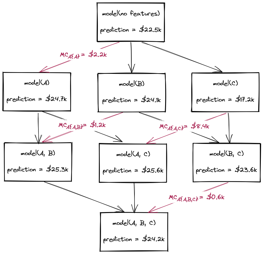
As explained previously, the Shapley values of a model can be computed exactly as a weighted sum of each feature's marginal contributions. This involves retraining the model 2F times, where \( F \) is the number of features. These retrained models encompass every possible combination of features, which in game theory terms, is referred to as the power set of all possible feature coalitions.
Training so many models is usually prohibitive, so instead we must find ways to approximate this process. In this section, we explore a naive approach for approximating Shapley values that avoids model retraining.
Reintroducing the dataset
We'll explore this idea using the same simplified version of the Boston housing dataset as used in the How Shapley Values Work post. This dataset contains the prices of 506 houses, accompanied by three predictive features (Table 1).
| Variable Name | Description |
|---|---|
| % working class | Percentage of the population that is working class. |
| number of rooms | The average number of rooms per house in the housing unit. |
| NOX concentration | Nitric oxides concentration (parts per 10 million). |
Table 1. The model input variables used to predict house prices.
Shapley values will enable us to understand the house price predictions of a machine learning model trained on these three features.
import numpy as np
import pandas as pd

features = ["% working class", "number of rooms", "NOX concentration"]
df = pd.read_csv("data.csv")
y = df["y"].values
print(f"{len(y)} rows")
print(df[features + ["y"]].sample(5, random_state=0))

# returns:
# 506 rows
#      % working class  number of rooms  NOX concentration        y
# 329            14.68            6.333              0.460  22600.0
# 371            19.06            6.216              0.631  50000.0
# 219            21.00            6.373              0.550  23000.0
# 403            39.54            5.349              0.693   8300.0
# 78             24.68            6.232              0.437  21200.0
Training the Model
Whereas before we had to train \( 2^3 = 8 \) models, this time, we only need to train the model we're ultimately interested in: the one that uses all three features.
from sklearn.ensemble import RandomForestRegressor

X = df[features]
model = RandomForestRegressor(random_state=0).fit(X, y)
y_pred = m.predict(X)
Generating marginalised predictions
Our naive approximation approach is to use this single model for the entire power set, but for each feature that's missing in a given feature coalition, we randomly replace that feature's value with another value from the dataset. In SHAP, "removing" features using methods such as this is referred to as masking.
The function below shows what this looks like for a model generating a prediction for a single row in a pandas DataFrame.
def marginalised_prediction(row, m=model, X=X, missing=[]):
    """Generate a prediction for `row` using model `m`, replacing
    features in `missing` by sampling randomly from `X`."""
    instance = row.copy()
    for feature in missing:
        instance[feature] = np.random.choice(X[feature])
    return m.predict([instance])
Replacing the value of a feature with another value sampled at random from the dataset is referred to as sampling from the feature's marginal distribution. This can result in unrealistic combinations of feature values. More sophisticated methods will sample from the conditional distribution, which ensures that only realistic feature combinations are yielded. But we'll make do with the marginal distribution for now.
Generating a prediction for a coalition that has only sampled each missing feature once will give highly variable results. To obtain consistent predictions, we average this process over a large number of samples, as follows:
def approximate_prediction(row, m=model, X=X, missing=[], n=100):
    """Average the results returned by `marginalised_prediction()`
    over `n` predictions."""
    predictions = []
    for _ in range(n):
        predictions.append(marginalised_prediction(m, X, row, missing))
    return np.mean(predictions)
We can now compute the marginal contributions of each feature in an analogous manner to how we did when we computed them exactly via model retraining. We use the approximate_prediction() function to generate marginalised predictions for every instance in the dataset, across all eight feature coalitions. This corresponds to one coalition with zero features (for which the predictions will be equal to the average house price in the dataset), three coalitions with one feature, three coalitions with two features, and one coalition with all three features (i.e. the model we're interested in).
predictions = {}

# predictions with no features
predictions["none"] = X.apply(
    lambda row: approximate_prediction(
        row,
        missing=features
    ),
    axis=1
)

# predictions with one feature
for feat in features:
    predictions[feat] = X.apply(
        lambda row: approximate_prediction(
            row,
            missing=[c for c in features if c != feat]
        ),
        axis=1
    )

# predictions with two features
for i, feat1 in enumerate(features):
    for feat2 in features[i+1:]:
        predictions[f"{feat1}, {feat2}"] = X.apply(
            lambda row: approximate_prediction(
                row,
                missing=[c for c in features if c not in [feat1, feat2]]
            ),
            axis=1
        )

# predictions with all features
predictions["all"] = m.predict(X)
Approximating the features' Shapley values
Finally, we approximate the Shapley values of each feature using the same weighted averages as before. To understand this calculation, see The Mechanics of Shapley Values.
sv_pwc = 1/3 * (predictions["% working class"] -
                predictions["none"]) +\
         1/6 * (predictions["% working class, number of rooms"] -
                predictions["number of rooms"]) +\
         1/6 * (predictions["% working class, NOX concentration"] -
                predictions["NOX concentration"]) +\
         1/3 * (predictions["all"] -
                predictions["number of rooms, NOX concentration"])

sv_nor = 1/3 * (predictions["number of rooms"] -
                predictions["none"]) +\
         1/6 * (predictions["% working class, number of rooms"] -
                predictions["% working class"]) +\
         1/6 * (predictions["number of rooms, NOX concentration"] -
                predictions["NOX concentration"]) +\
         1/3 * (predictions["all"] -
                predictions["% working class, NOX concentration"])

sv_nc  = 1/3 * (predictions["NOX concentration"] -
                predictions["none"]) +\
         1/6 * (predictions["% working class, NOX concentration"] -
                predictions["% working class"]) +\
         1/6 * (predictions["number of rooms, NOX concentration"] -
                predictions["number of rooms"]) +\
         1/3 * (predictions["all"] -
                predictions["% working class, number of rooms"])
We can now used our approximated Shapley values to quantify the average impact of each feature on the model's house price predictions.
print("Mean absolute shapley values:")
print(f"% working class  : {np.abs(sv_pwc).mean():,.1f}")
print(f"number of rooms  : {np.abs(sv_nor).mean():,.1f}")
print(f"NOX concentration: {np.abs(sv_nc).mean():,.1f}")

# Returns:
# Mean absolute shapley values:
# % working class  : 4,051.3
# number of rooms  : 2,695.0
# NOX concentration: 1,289.9
Is this actually better than what we had before?
We've successfully estimated Shapley values without having to do any model retraining, but the astute reader has probably realised that we've just replaced one computationally intensive process with another. In fact, the above code - which prioritises clarity over efficiency - is much slower than the exact calculation of Shapley values demonstrated previously.
This leads us to SHAP, which encompasses various methods that leverage clever masking strategies to approximate Shapley values more efficiently than the naive approach outlined above.
 AidanCooper
Code for this walkthrough can be found on GitHub
Member discussion