Dec 31, 2022 10 min read Explainable AI

How Shapley Values Work

In this article, we will explore how Shapley values work - not using cryptic formulae, but by way of code and simplified explanations

Shapley values - and their popular extension, SHAP - are machine learning explainability techniques that are easy to use and interpret. However, trying to make sense of their theory can be intimidating. In this article, we will explore how Shapley values work - not using cryptic formulae, but by way of code and simplified explanations.

Introducing the Dataset

Before we dive into things, we'll briefly examine the dataset that will be used throughout this post.

We'll calculate Shapley values from scratch using a simplified version of the Boston housing dataset. This dataset contains the prices of 506 houses, accompanied by three predictive features (Table 1).

Variable Name	Description
% working class	Percentage of the population that is working class.
number of rooms	The average number of rooms per house in the housing unit.
NOX concentration	Nitric oxides concentration (parts per 10 million).

^{Table 1. The model input variables used to predict house prices.}

Shapley values will enable us to understand the house price predictions of a machine learning model trained on these three features.

import pandas as pd

features = ["% working class", "number of rooms", "NOX concentration"]
df = pd.read_csv("data.csv")
y = df["y"].values
print(f"{len(y)} rows")
print(df[features + ["y"]].sample(5, random_state=0))

# returns:
# 506 rows
#      % working class  number of rooms  NOX concentration        y
# 329            14.68            6.333              0.460  22600.0
# 371            19.06            6.216              0.631  50000.0
# 219            21.00            6.373              0.550  23000.0
# 403            39.54            5.349              0.693   8300.0
# 78             24.68            6.232              0.437  21200.0

The Mechanics of Shapley Values

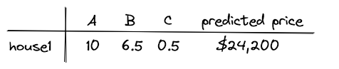
Suppose we have a machine learning model, $ model(A,B,C) $, which has been trained on the above dataset to predict house prices based on three features, $ A $, $ B $, and $ C $. We select an instance from the dataset, $ house1$, with feature values $ A=10 $, $ B=6.5 $, and $ C=0.5 $. The model predicts a price of $24,200 for $ house1$.

The Shapley values for $ house1$ will quantify how much each of its features contributes to the predicted price, $ p(house1)$, of $24,200. This is expressed by the following relationship, where the base value, $ b$, is a fixed constant that is the same across all instances in the dataset:

$$ p(house1) = b + shapley_A(house1) + shapley_B(house1) + shapley_C(house1) $$

To calculate these Shapley values for features $ A $, $ B $, and $ C $, we must consider the power set of all possible feature coalitions. This is a fancy way of saying: consider all possible combinations of the three features, spanning 0, 1, 2, and all 3 features. For each coalition, we retrain the machine learning model using the features included in the coalition. This power set of models is shown in Figure 1, with the models connected from top to bottom by the incremental addition of features. For the model trained on no features, the prediction is always the average house price in the dataset. This constant prediction is the previously mentioned base value (in this example, $22,500).

The Shapley values are based on the marginal contributions of each feature to the models' predictions. That is to say, for $ house1$, what is the change in predicted price when a feature is added to the model? Figure 1 illustrates the marginal contributions of feature $ A $, denoted in red as $ MC_A $.

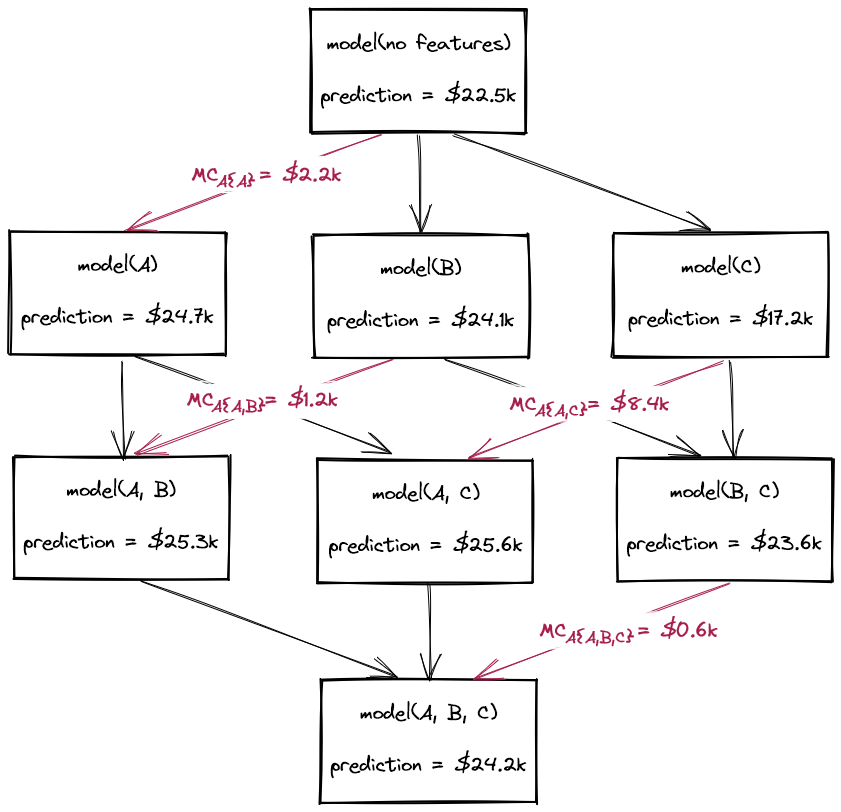
**Fig 1.** The power set of models using features $ A$, $ B$, and $ C$, with predictions for $ house1$. Exemplified in red are the marginal contributions of feature $ A$.

From these marginal contributions, we can calculate the Shapley value of feature $ A $ for $ house1 $ as a weighted sum of the marginal contributions. The weights are the reciprocal of the count of connections at each layer. Note that the weights sum to 1.

$$ shapley_A(house1) = 1/3 \times 2200 + 1/6 \times 1200 + 1/6 \times 8400 + 1/3 \times 600 $$

For feature $ A $, this calculates a Shapley value of $2,550 for $ house1 $. The equivalent calculations for features $ B $ and $ C $ produce Shapley values of $1,250 and -$2,100, respectively. The relationship between the predicted price and Shapley values holds true: $24,200 = 22,500 + 2,550 + 1,250 - 2,100$.

From these Shapley values, we can see that $ house1 $'s feature values of $ A=10$ and $ B=6.5 $ are contributing towards a higher than average predicted house price, whereas $ C=0.5$ pushes the prediction downwards. By calculating the three features' Shapley values for all houses in the dataset, we can reveal insights into how the machine learning model makes its predictions.

A Note on Shapley Values versus SHAP Values

Shapley values and SHAP values are often conflated, but they aren't exactly the same. SHAP encompasses a range of techniques for efficiently approximating Shapley values, by combining them with local interpretability methods such as LIME. This complicates the mechanics of SHAP, but it provides some major advantages in return:

To calculate Shapley values, you must retrain your machine learning model 2^F times (where F is the number of features). SHAP avoids this by using approximation methods, making it viable for applications where obtaining Shapley values would be computationally infeasible.
Although SHAP can be applied to any machine learning model, for tree-based models, SHAP uses an algorithm that is especially fast at estimating Shapley values.

For a gentle introduction to SHAP analyses, I recommend checking out a previous post of mine:

Although standard Shapley values are largely obsolete to those produced by SHAP for most use cases, the theory carries over, so it's still useful to understand. I'll explain how SHAP works in a future post, so subscribe if that's something you'd like to see.

Subscribe for more posts like this

Calculating Shapley Values: A Worked Example

This worked example has three stages:

Retraining the machine learning model for each feature coalition.
Calculating the Shapley values from each feature's marginal contributions.
Visualising the Shapley values to generate insights.

Train the Machine Learning Models and Make Predictions

We want to obtain Shapley values for the machine learning model trained on all three features. As we saw in the theory section, this requires us to retrain the model 2³ times, for the full power set of possible feature coalitions. This is shown in the code sample below, where a model is trained for each possible combination of features and stored in the models dictionary. This includes the full feature model, models["all"], that we're ultimately interested in.

from sklearn.ensemble import RandomForestRegressor

models = {}

# model with no features
models["none"] = [y.mean()] * len(y)

# models with one feature
for feature in features:
    X = df[feature].values.reshape(-1, 1)
    m = RandomForestRegressor(random_state=0).fit(X, y)
    models[feature] = m.predict(X)

# models with two features
for i, feature1 in enumerate(features):
    for feature2 in features[i+1:]:
        X = df[[feature1, feature2]].values
        m = RandomForestRegressor(random_state=0).fit(X, y)
        models[f"{feature1}, {feature2}"] = m.predict(X)

# model with all features
X_all = df[features]
m = RandomForestRegressor(random_state=0).fit(X_all, y)
models["all"] = m.predict(X_all)

In this example, we're using a random forest model with scikit-learn's default hyperparameters. In most real-world applications, you would arrive at a set of custom hyperparameters for your model trained on all the features via tuning. These hyperparameters would then be held constant during the retraining of the model.

Calculate the Shapley Values

Now that we have our power set of models, we can calculate the Shapley values as the weighted average of the marginal contributions for each feature.

sv_pwc = 1/3 * (models["% working class"] -
                models["none"]) +\
         1/6 * (models["% working class, number of rooms"] -
                models["number of rooms"]) +\
         1/6 * (models["% working class, NOX concentration"] -
                models["NOX concentration"]) +\
         1/3 * (models["all"] -
                models["number of rooms, NOX concentration"])

sv_nor = 1/3 * (models["number of rooms"] -
                models["none"]) +\
         1/6 * (models["% working class, number of rooms"] -
                models["% working class"]) +\
         1/6 * (models["number of rooms, NOX concentration"] -
                models["NOX concentration"]) +\
         1/3 * (models["all"] -
                models["% working class, NOX concentration"])

sv_nc  = 1/3 * (models["NOX concentration"] -
                models["none"]) +\
         1/6 * (models["% working class, NOX concentration"] -
                models["% working class"]) +\
         1/6 * (models["number of rooms, NOX concentration"] -
                models["number of rooms"]) +\
         1/3 * (models["all"] -
                models["% working class, number of rooms"])

Here, sv_pwc, sv_nor and sv_nc are arrays containing 506 elements - each being that feature's Shapley value for each instance in the dataset.

Create a Waterfall Chart for a Single Instance

We'll now visualise these Shapley values to generate insights into the workings of our machine learning model.

A common SHAP plot for understanding local feature importance (i.e. how features contribute to the prediction of a single instance in the dataset) is the waterfall chart. This deconstructs a single house's prediction into the base value, plus the SHAP values for each feature of that house. We can create waterfall charts using plotly.

import plotly.graph_objects as go

i = 0
fig = go.Figure(
    go.Waterfall(
        name="waterfall",
        orientation="h",
        y=features,
        x=[sv_pwc[i], sv_nor[i], sv_nc[i]],
        base=models["none"][i],
        decreasing=dict(marker=dict(color="#008bfb")),
        increasing=dict(marker=dict(color="#fb0655"))
    )
)
fig.update_layout(
    title=f"Base: &#36;{models['none'][i]:,.0f}, Prediction: &#36;{models['all'][i]:,.0f}",
    width=1000, height=500, font=dict(size=14),
)
fig.write_image("plots/waterfall.png")

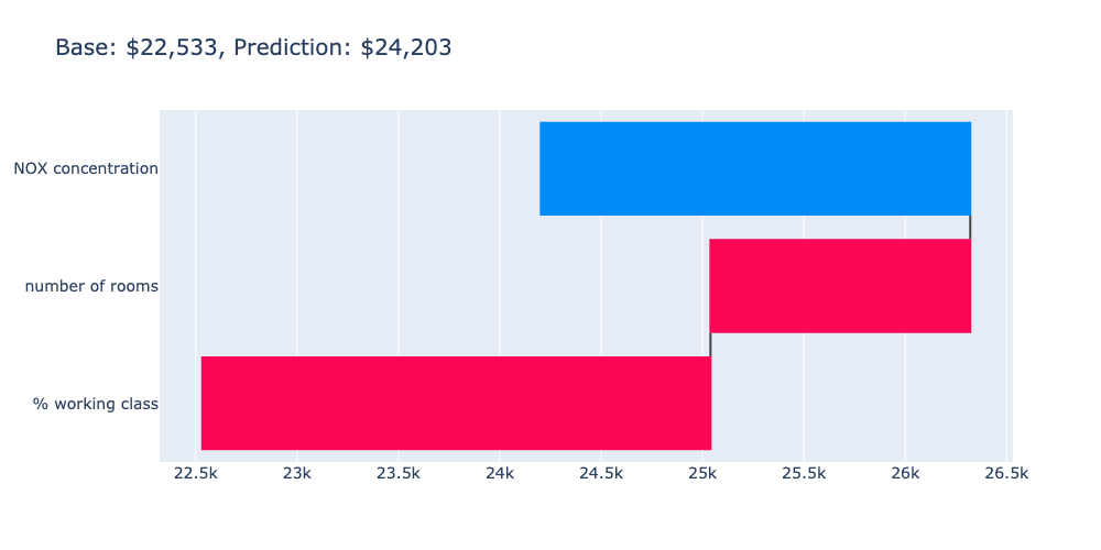
For this particular example using the first instance in the dataset ($i=0$), we see that the % working class and number of rooms features "push" the house price prediction higher to ~$26,300 from the starting point (base value) of $22,533. The NOX concentration feature, however, reduces it to a final value of $24,203. The base value is the mean house price in the dataset, which is stored in models["none"] ($22,532).

We can verify that the sum of the base value and Shapley values equal the house price predictions for all houses in the dataset using np.all(np.isclose(models["none"] + sv_pwc + sv_nor + sv_nc, models["all"])), which returns True.

Create a Bar Chart of the Mean Absolute Shapley Values

To understand the global importance of the model's features, we'll create a bar chart of the mean absolute Shapley values (MASVs). This is a measure of how much each feature influences the model's house price predictions, on average. The MASVs are calculated and plotted using the code below.

import matplotlib.pyplot as plt

fig, ax = plt.subplots()
ax.barh(
    ["NOX concentration", "number of rooms", "% working class"],
    [np.abs(sv_nc).mean(), np.abs(sv_nor).mean(), np.abs(sv_pwc).mean()],
    height=0.6,
)
ax.grid(axis="x")
ax.set_xlabel("mean absolute shapley value")

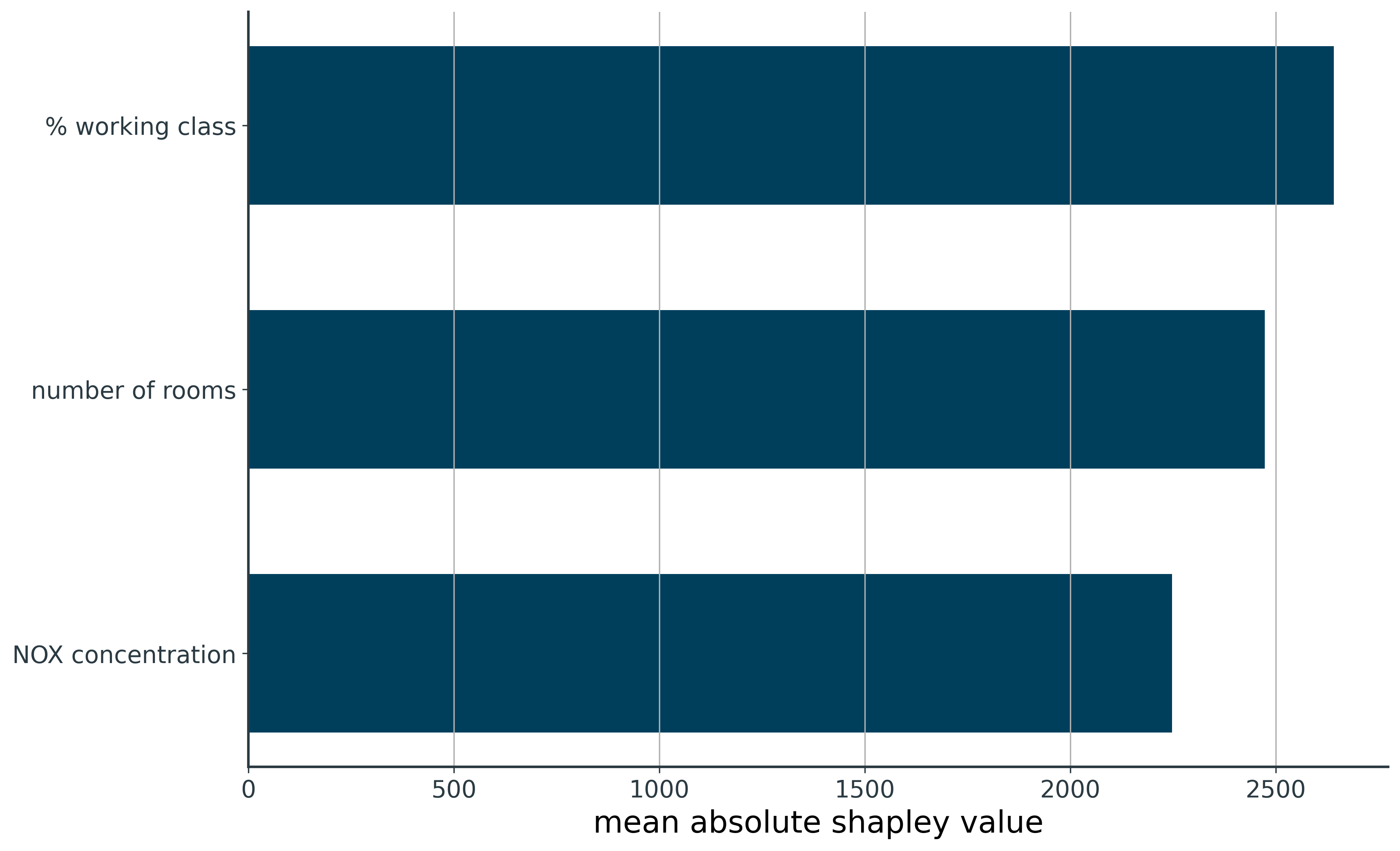
We see that on average, % working class, number of rooms, and NOX concentration, contribute ±$2,641, ±$2,474, and ±$2,247 to each house price prediction, respectively.

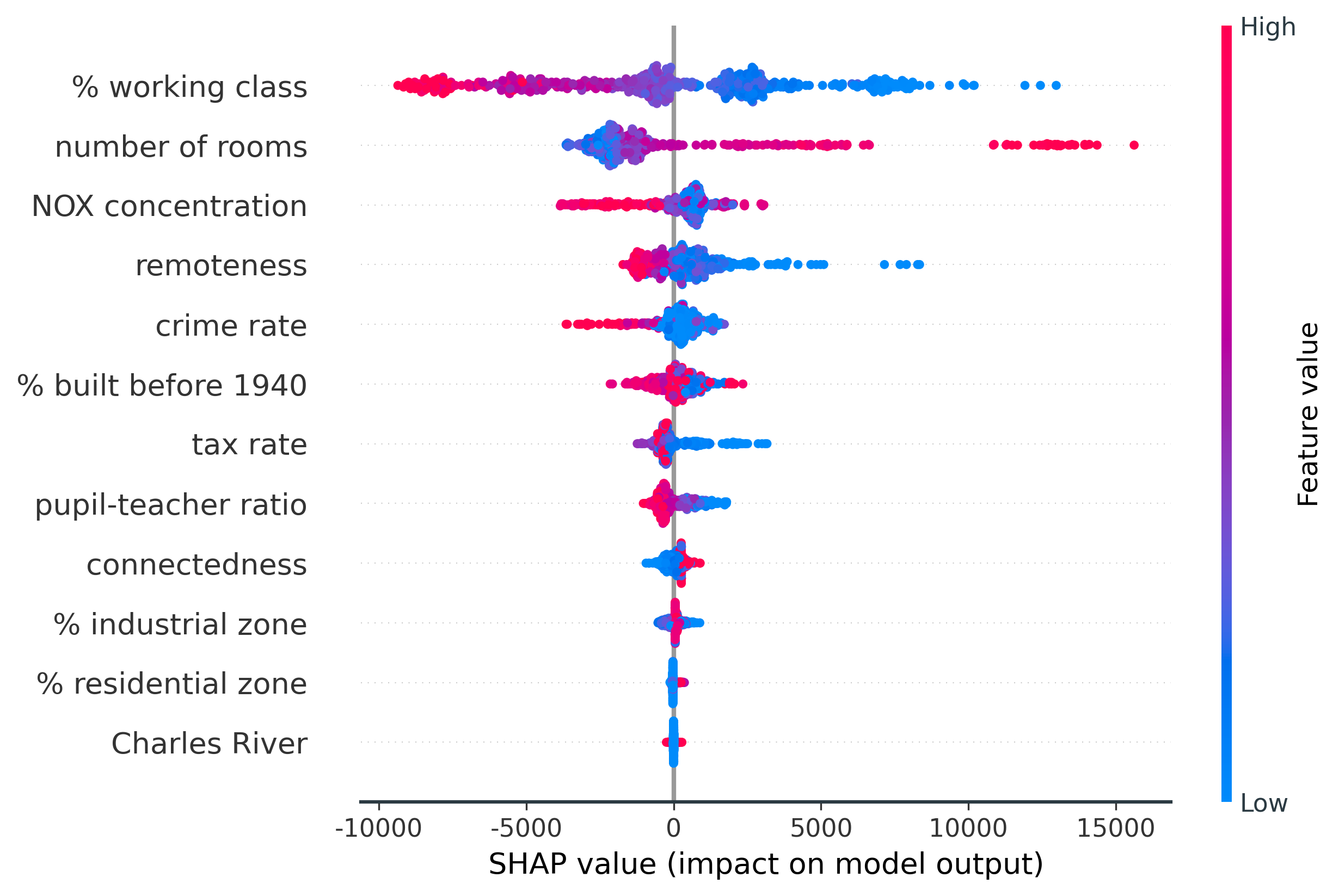
Create a Beeswarm Plot of the Shapley Values

Another useful representation of Shapley values is the beeswarm plot. This allows us to see the full distribution of Shapley values for each feature, and understand their relationships with the actual feature values. The code below uses the seaborn library to produce the beeswarm plot.

import seaborn as sns

# shape data for beeswarm plot
df_sv = pd.DataFrame()
df_sv["feature"] = (
    ["% working class"] * len(y)
    + ["numer of rooms"] * len(y)
    + ["NOX concentration"] * len(y)
)
df_sv["shapley value"] = np.concatenate([sv_pwc, sv_nor, sv_nc])
df_sv["hue"] = np.concatenate(
    [
        (df["% working class"].values - df["% working class"].mean())
        / df["% working class"].std(),
        (df["number of rooms"].values - df["number of rooms"].mean())
        / df["number of rooms"].std(),
        (df["NOX concentration"].values - df["NOX concentration"].mean())
        / df["NOX concentration"].std(),
    ]
)

# beeswarm plot
fig, ax = plt.subplots()
ax.axvline(0, c="grey", alpha=0.8)
ax = sns.swarmplot(
    x=df_sv["shapley value"],
    y=df_sv["feature"],
    hue=df_sv["hue"],
    palette="coolwarm",  # red = higher raw value; blue = lower raw value
    size=5,
    legend=False,
)
ax.spines.left.set_visible(False)
ax.grid(axis="x")
ax.set_ylabel("")
fig.savefig("plots/beeswarm.png")

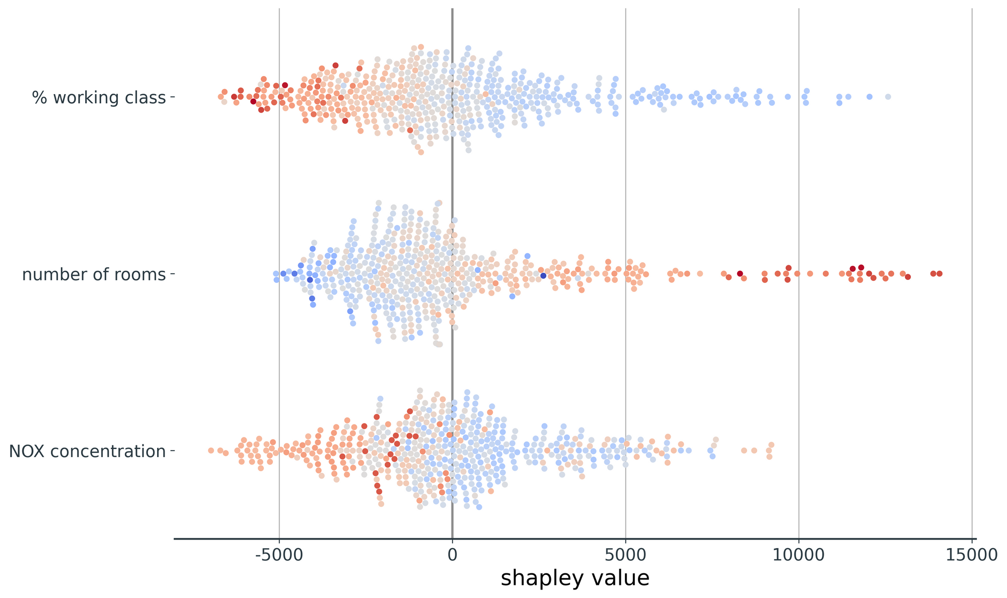
Here are two insights we can infer from the beeswarm plot:

Lower values of % working class (blue dots) have positive Shapley values (i.e. contribute towards predictions of higher house prices). The same is (generally) true of NOX concentration, and the opposite is true of number of rooms.
The largest Shapley values (~$14,000) are seen for high values (red dots) of the number of rooms feature.

Conclusion

In this article, we've calculated Shapley values from scratch for a three-feature random forest regressor. We've also seen how these Shapley values can be visualised to generate insights into the predictions of the model.

In a future posts, we'll explore how Shapley values are extended for practicable application to machine learning using SHAP. The next article explains how Shapley values can be approximated for machine learning models, instead of using the computationally intensive exact calculation outlined in this post.

Subscribe for future posts on SHAP